Kepler Exoplanet Detection
Binary Classification for Exoplanet Detection
This project was based on a dataset provided by NASA from the Kepler Space Telescope, which operated from 2009 to 2018. We chose this project due to the increasing popularity of space travel after SpaceX’s successful catch of the Super Heavy Rocket. The goal of the project was to be able to classify whether a object in space was considered as an exoplanet or not. With the amount of data and measurements taken, we hoped to be able to expedite the process for astronomists.
Our data consisted of 9576 objects of interest (these are referenced as koi or Kepler Objects of Interest) with 49 different features that included things like the object’s transit properties, star parameters, and parameters on the crossing event. I began by creating a correlation heatmap. Initially, I removed many of the features that had to do with identification of the object or features that were archived or leaked information on whether the object was an exoplanet or not (leading to 13 dropped columns). Our target variable was the koi_pdisposition column, which was a binary column of CANDIDATE or FALSE POSITIVE on whether the object was an exoplanet or not. This was then binary encoded for use in the model later. For the remaining features, we split the dataset into train, test, and validation sets for later use.
Exploratory Data Analysis and Feature Engineering
The first observation I made was that many of the features has error columns which had the positive and negative errors of that feature’s measurement. However, these error columns had perfect correlation with the measurements themselves due to the fact that error increases proportionally with any measurement taken. Therefore, to remove collinearity and redundancy of features, I dropped all of the columns. The reduced heatmap is shown below, now with 16 measurement features.

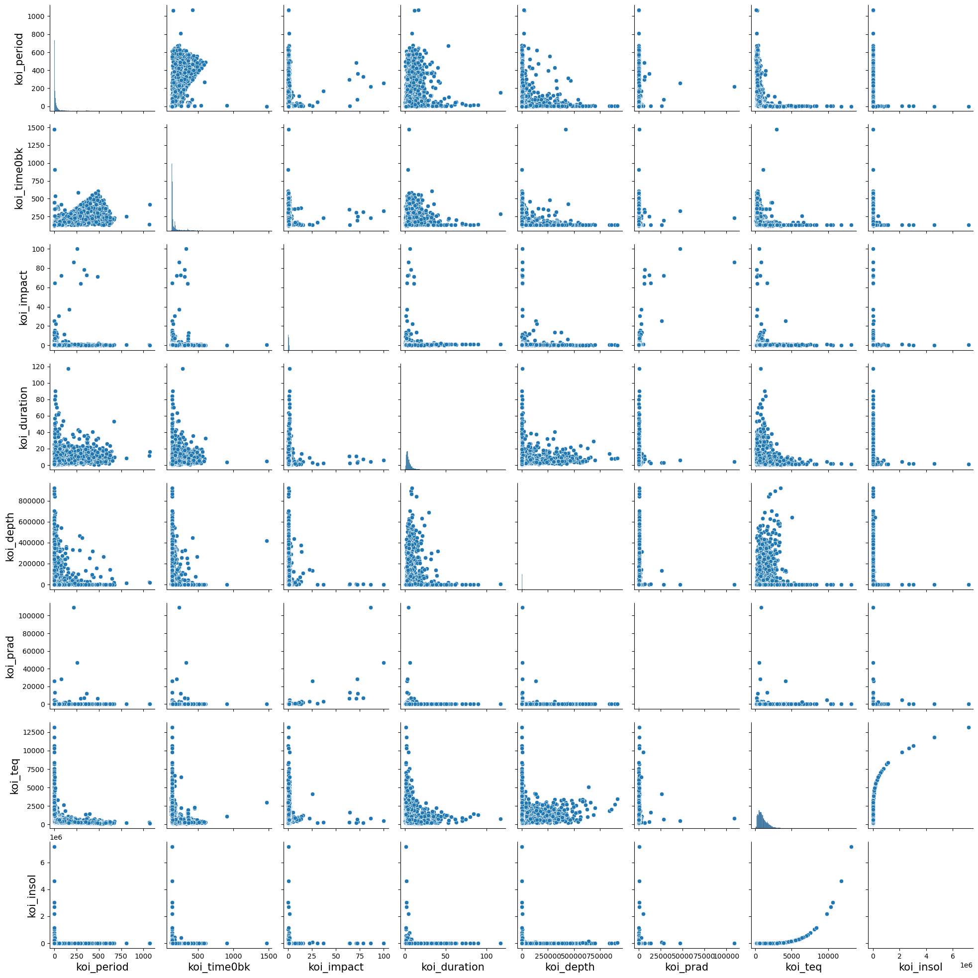
Next we reviewed the pairplot between all features. Due to the sheer number of features remaining, I split the features into different categories: Stellar Parameters (features on the star that the object orbits around), Threshold Crossing Event features (a.k.a. TCE, which is the event when the planet blocks some amount of light from the star that is detectable and marks an object of interest), and Transit Properties (or the properties about the object and its orbit). The below pairplot shows all the features belonging to the transit properties of the objects.

From the pairplot I observed that most of the histograms along the diagonal showed that nearly all of the features were heavily right skewed (some were so skewed that I couldn’t even see it on the histogram). Also another observation was that there were several features that showed some form of logarithmic relationship between them, as seen from the scatterplot between koi_insol and koi_teq. Both of these observations meant that I should transform these numeric features to better capture relationships as well as to reduce the effect of outliers. As a result, I log-transformed all of the numeric variables. The only one where I did not transform was the koi_tce_plnt_num, as this was a label_encoded value from 1-8. The planet number will be one hot encoded later.
# copy all of the data sets for log transformations
X_train_log = X_train.copy()
X_val_log = X_val.copy()
X_test_log = X_test.copy()

# column names that need log transformations
log_transform_columns = transit_prop_columns + ['koi_model_snr', 'koi_srad']

# log transform all of the columns listed above
X_train_log[log_transform_columns] = X_train_log[log_transform_columns].apply(np.log1p)
X_val_log[log_transform_columns] = X_val_log[log_transform_columns].apply(np.log1p)
X_test_log[log_transform_columns] = X_test_log[log_transform_columns].apply(np.log1p)
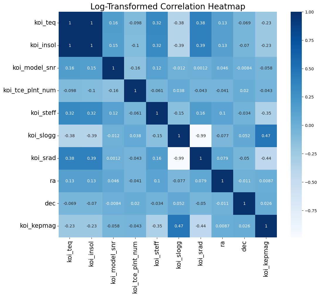
From here, I replotted the heatmap with the log transformed values along with the pairplot. As seen from the pairplot most of the distributions were now more visible and some of the features had a more normal distribution. Also, after log transformation, we see that koi_teq and koi_insol were now nearly linear after log transforming all the features. This is further emphasized in the correlation heatmap, which shows that koi_teq and koi_insol have a 1.0 correlation with one another. Investigating these two variables further, the NASA data dictionary does state that the koi_teq is the equilibrium temperature of the object while the koi_insol is the insolation flux, or the radiation heatflux of the object. This makes sense as the heat flux caused by radiation is proprotional to the Temperature to the fourth power (q ⍺ T4). As a result, when we log transformed both variables, we get a perfectly linear relationship.
The same goes for the -0.99 corrleation between koi_slogg and koi_srad, which is the gravitational acceleration and the radius of the star, respectively. The gravitational acceleration is inversely proportional to the radius of the star squared (g ⍺ r-2), which is why we see the negative correlation after log transformation. As a result of these findings, we removed koi_srad and koi_insol to avoid redundancy between variables.


For a final observation, I saw that after log transformations, there were several features that had bimodal distributions after separating by classes. For each of these, we attempted to bin the features in order to separate the peaks and allow for easier classification; however, we observed from modelling, that it ended up reducing our overall accuracy of all of our models. This could be due to the fact that we are over simplifying the relationship. As a result, the manual binning process is displayed in the code, but we did not end up using this bit of feature engineering.

Some final preprocessing with the data was that we used a RobustScalar to standardize the data. We used a RobustScalar in order to scale outliers better, since even with the log transformations, we still observed some outliers in some of our features. As for missing values, we ended up dropping missing values which consisted of 4%, 3$, and 2% in our train, validation, and test datasets respectively. Due to the low percentage, we assumed that we’d have enough data for modelling. Also, we had two categorical variables (koi_tce_plnt_num and koi_tce_delivname) which had eight and three categories, respectively. This led us to one hot encoding these two columns. In conclusion, we ended up with 8945 rows and 24 total features.
Baseline Models
We ran two different baseline models in order to compare our final model to. The first was a linear regression with cross validation.
# create logistic regression model
linear_model = LogisticRegression()

# use cross validation for determining scores
cv_scores = cross_val_score(linear_model, X_train_final, y_train_final, cv=5)

# Test logistic regression model on validation set
linear_model.fit(X_train_final, y_train_final)
y_val_pred = linear_model.predict(X_val_final)
This resulted in a cross-validated mean accuracy of 80.4%. Afterward, we made a random forest classifier with 200 esimators. This resulted in a mean cross validation accuracy of 83.5%.
# Model with best parameters
rf_model = RandomForestClassifier(n_estimators=200, max_depth=20, max_features='sqrt',
                                  min_samples_split=2, min_samples_leaf=1)

rf_model.fit(X_train_final, y_train_final)

rf_cv_scores = cross_val_score(rf_model, X_train_final, y_train_final, cv=5)
Both of these accuracies did pretty well for the simplicity of implementation. We ultimately decided to see if a neural network improved upon these two baselines.
Final Model
We ultimately chose to do a neural network to better capture the nonlinear relationships and be able to optimize the hyperparameters. Also our training dataset is ~5000 datapoints; however, with more data we could find online, we may be able to improve the training on this model over time. As a result, after trial and error, we ultimately ended up with a feed forward neural network with one input layer, three hidden layers with ReLU activation, two dropout layers (with dropout rate = 0.3), and an output layer with softmax activation. Other hyperparameters included a 0.00001 learning rate, Adam optimizer, 32 batch size, and 1000 epochs with EarlyStopping callback (patience of 10 epochs).

This final model ultimately resulted in a 84.2% validation accuracy, which we were satisfied with for the purposes of this project. As a result, this ended up higher than our baseline models and so we went with this neural network. It can be argued that the neural network is comparable to the random forest model (with a difference in accuracy of 0.7%) to which I agree and we can ultimately choose either model for our final result. We again decided to go with the neural network to gain a better understanding with TensorFlow and potentially improve it further with more understanding of the features (as we are not experts in this field).
Model Evaluation
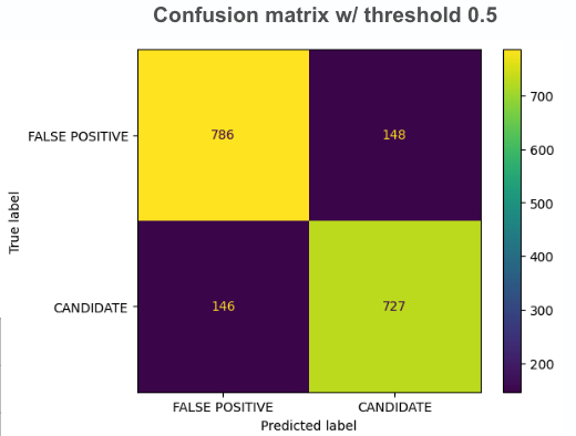
For our final evaluation, we used the test dataset to measure the metrics of accuracy, precision, and recall. The test dataset had an accuracy of 83.7%, which displayed that our model had relatively good generalization properties and could handle new data well. Also our F1-scores for False Positives and Candidate classifications was 84% and 83%, respectively, which once again showed that we were pretty balanced in the classification of both classes.d

Going back to the original goal, our task was to expedite the process of exoplanet classification; however, I thought that mislabeling the Candidate class as a False Positive class would lead to a much more serious impact, since then astronomists would have to rereview the candidate and false positive classes. As a result, we decided to decrease the decision threshold (from an initial threshold to 0.5). While this would make the Candidate class accuracy worse, it would ultimately improve our False Positive Accuracy and prevent misclassification of potential exoplanets getting scrapped into the False Positive Bin.
| Metric | Threshold=0.5 | Threshold=0.35 |
|---|---|---|
| Accuracy | 0.84 | 0.81 |
| Candidate Precision | 0.82 | 0.75 |
| Candidate Recall | 0.82 | 0.91 |
| False Positive Precision | 0.83 | 0.89 |
| False Positive Recall | 0.83 | 0.71 |
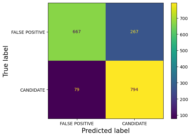
As seen from the table above, we decided on a threshold of 0.35, where it would lead to a 3% decrease in our overall accuracy, but it would improve our Candidate Recall and False Positive Precision to 91% and 89% respectively. This near 90% precision and recall significantly reduces the misclassification into the False positive bin as seen from the new confusion matrix below.

Conclusion
Ultimately, we decided on a Neural Network model with 84% test accuracy at a threshold of 0.5 and 81% test accuracy at a threshold of 0.35. Although we did some feature engineering and were able to find some interesting results that tied back to physics, we know there is so much more in the data to explore. If we were to have done this project with more time, we would ultimately looks further into each of the individual features and see how they interact with one another and tune our model to get an even better classification score. However, this project showed how we can use machine learning not just for software projects, but for real research, which we hope to utilize more with the revolutionization of artificial intelligence and machine learning.