Bank Transaction Classifier

Background and Motivation

This project is a machine learning project to be able to predict categories tailored to my specific bank transactions. Once I find the best machine learning model to predict my categories, I also delve into creating a locally hosted Dash app in order to easily upload new data, store the transactions, relabel the categories for said transactions, and retrain my model.

The motivation behind this project is to be able to easily create a budget based on how much I am spending on a regular basis. Although many institutions have good budget categorizers, I, like many other individuals, use multiple banks and apps for my finances. As a result, I wanted a centralized location that I could use to aggregate my transaction data and gain insights from it as a whole. Plus, the model would only see my data and so it will be customized for myself, which should allow it to better categorize my transactions.

The institutions I use are Bank of America (BofA), American Express (AmEx), and Venmo. Although BofA and AmEx are large banks that have their own personal categorization models, Venmo has very little data and thus it is difficult to know what I spend my money on through that app. We will utilize the categorizations that BofA and AmEx provide as well to hopefully enhance our model and allow it to learn all three institution’s transaction data in aggregation.

Transaction Storage

The initial data storage and processing can be reviewed through the clean transactions module. I first downloaded as many transaction statements as I could from my various banks and stored them in the transactions folder. From here, I created a SQLite database and used the same module to standarize the various instituions’ data. All three of the institutions had similar columns; however, they were all formatted differently and named differently.

In order to standardize the transactions, I chose to format the three institutions to be similar to American Express’s data as it included more columns that the other banks did not (such as merchant address, city, state, etc.). We will breifly go over Venmo’s transaction data processing as it required the most changes.

First, I checked the NaN columns and dropped several columns that had 100% nan values. I also deleted columns that had the same values for every single transaction.

def calc_nan_percent(df):
    """Calculate the % of nan values in each column of a DataFrame"""
    return df.isna().sum(axis=0)/df.shape[0]

# drop amount_(tax), tax_rate because they are all empty strings or no value added
# drop destination and funding_source b/c mostly all null and theres not value added
drop_columns = ['amount_(tax)', 'tax_rate', 'destination',
                'funding_source','destination']

venmo_nan = calc_nan_percent(venmo_df)

# drop columns that have only null values + the list above
venmo_df = venmo_df.drop(columns = list(venmo_nan[venmo_nan == 1].index) + drop_columns)

Then I created a function to alter the amount column to make it suitable as a float instead of a string. Venmo data included many non-numeric characters, like “($1,526.77)” that could not be converted directly into a float value. Also the amount of the transaction was always positive and the only way to know whether the transaction was income or a charge was to review the type and from columns in conjunction. As a result, I made the amount negative if the type was a ‘Payment’ and it came from myself to indicate that it was money that I spent. Finally, to make the data more compact, I made any transfers to my bank as part of the note column instead of the type column so I could drop the type column.

def extract_amount(row):
    """regex to extract the amount as a float instead of a string."""
    # delete commas, parenthesis and whitespace
    amount = float(re.sub(r'\$|,|\(|\)| ','',row['amount']))
    
    # check if I paid the person, then make it negative
    if row['type'] == 'Payment' and row['from'] == 'Kenneth Hahn':
        amount = -1*abs(amount)

    # if it's a transfer to my bank, then make the note the Standard Transfer type (description)
    note = row['note']
    if row['type'] == 'Standard Transfer':
        note = 'Standard Transfer'

    return pd.Series([note, amount], index=['note', 'amount'])

venmo_df[['note','amount']] = venmo_df.apply(extract_amount, axis=1)

Finally, I renamed the columns to match the other data and I dropped all the redundant columns that were not used or combined with other features.

# rename columns to match amex data
venmo_df = venmo_df.rename(columns={'datetime':'date',
                                    'note':'description',
                                    'terminal_location':'source'
                                    })

# convert datetime to date object
venmo_df['date'] = pd.to_datetime(venmo_df['date']).dt.date

# create new column to match amex data
venmo_df['extended_details'] = 'from ' + venmo_df['from'] + ' to ' + venmo_df['to'] 

# drop redundant columns
venmo_df = venmo_df.drop(columns=['from','to','type','status','id'])

Once all three of the DataFrames were processed and ready for storage, I concatenated all three tables and created a unique id for each of the transactions. This is used as the primary key for the data and it uses the date, amount, details, and source of the transaction (where source is the bank or institution where the transaction comes from). With this primary key, the transaction data is imported into the transactions.db SQLite database.

############################################################################################
#                      Concatenate and Create Unique IDs                                   #
############################################################################################

combined_df = pd.concat([boa_df, amex_df, venmo_df], ignore_index=True)

def create_transaction_id(row):
    """Get unique columns to combine and return a unique id"""
    unique_string = f"{row['date']}_{row['amount']}_{row['extended_details']}_{row['source']}"
    return hashlib.sha256(unique_string.encode()).hexdigest()

combined_df['transaction_id'] = combined_df.apply(create_transaction_id, axis=1)

############################################################################################
#                      Insert into transactions Database                                   #
############################################################################################

def insert_db(df, conn):
    cursor = conn.cursor()
    insert_query = '''
    INSERT OR IGNORE INTO transactions (
        transaction_id,
        date,
        description,
        extended_details,
        amount,
        source,
        merchant,
        address,
        city,
        state,
        zip_code,
        category
    ) VALUES (?, ?, ?, ?, ?, ?, ?, ?, ?, ?, ?, ?)
    '''

    for _, row in df.iterrows():
        cursor.execute(insert_query, (
            row['transaction_id'],
            row['date'],
            row['description'],
            row['extended_details'],
            row['amount'],
            row['source'],
            row['merchant'],
            row['address'],
            row['city'],
            row['state'],
            row['zip_code'],
            row['category']
        ))

    conn.commit()

insert_db(combined_df, conn)
conn.close()

Feature Engineering

Once I had the data stored in a database, I needed to further preprocess to be useable for a model. To review the preprocessing steps thoroughly, please review the model_selection_notebook for the detailed justification on steps. Also, to view how I made the data preprocessing into a Pipeline for app use, please review the custom_preprocessors module.

Target Variable

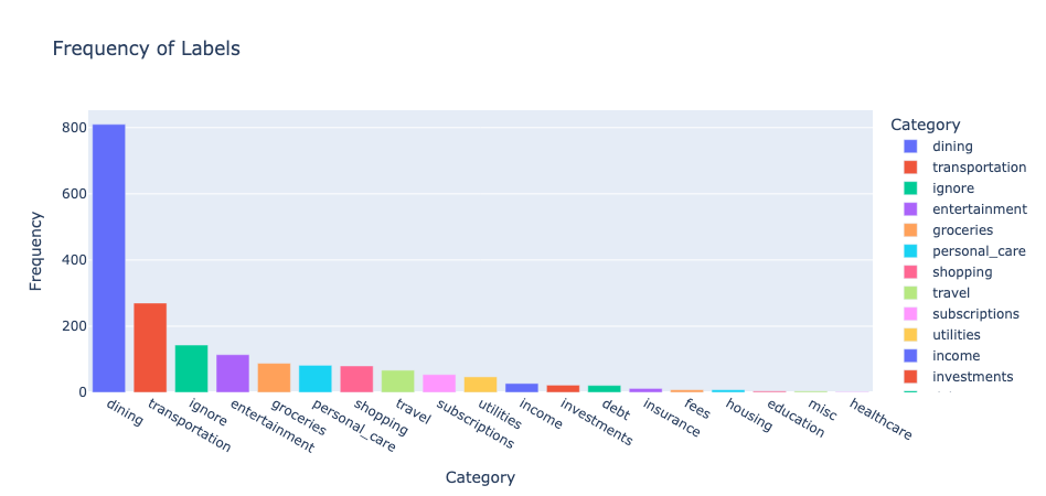
For the target variable labels, I one hot encoded the variable using LabelBinarizer, ending up with 19 distinct categories for transactions. By reviewing the class distribution below, I saw that the classes are extremely imbalanced; however, I only had 1047 rows available for training data. As a result, I decided to just leave the classes as is. As we’ll see with the final model, the model still does relatively well overall and some confusion with some of the categories won’t impact my budgeting significantly.

Numeric and Datetime Features

Moving onto the features, I started with processing the date feature. Because a lot of information can be extracted from the date of the transaction (such as a subscription payment or a weekly payment), I decided to split up the date into multiple features: the day of the week (dow), the day of the month (dom), the month, and the year. From these new columns, I decided to cyclically encode the day of the week and the month so the model can learn the cyclical nature of the dates to capture any regularly scheduled purchases. For the dom, I used StandardScaler to normalize the data and for the year I one hot encoded the years, since there were very few years in the data.

# use cyclic encoding to encode the cyclic nature of days of the week and month
shuffled_txns_df['dow_sin'] = np.sin(2 * np.pi * shuffled_txns_df['dow'] / 7)
shuffled_txns_df['dow_cos'] = np.cos(2 * np.pi * shuffled_txns_df['dow'] / 7)

shuffled_txns_df['month_sin'] = np.sin(2 * np.pi * shuffled_txns_df['month'] / 12)
shuffled_txns_df['month_cos'] = np.cos(2 * np.pi * shuffled_txns_df['month'] / 12)

# one hot encode the year and source
encoder = OneHotEncoder(sparse_output=False)
year_encoded = encoder.fit_transform(shuffled_txns_df[['year','source']])
year_encoded_df = pd.DataFrame(year_encoded, columns=encoder.get_feature_names_out(['year','source']))
shuffled_txns_df = pd.concat([shuffled_txns_df.drop(columns=['year','source']), year_encoded_df], axis=1)

# split the data 
X_train, X_temp, y_train, y_temp = train_test_split(shuffled_txns_df, y_onehot, test_size=0.4, random_state=42)
X_val, X_test, y_val, y_test = train_test_split(X_temp, y_temp, test_size=0.5, random_state=42)

# Scale 'dom' and 'year' using StandardScaler
scaler = StandardScaler()
scale_columns = ['dom']

As for our only numeric feature amount, I decided to use a RobustScaler instead as the transaction amounts vary widely and the RobustScaler is more robust toward outliers.

# Use RobustScaler to scale and replace the 'amount' column
robust_scaler = RobustScaler()
amount_train = pd.Series(robust_scaler.fit_transform(X_train[['amount']]).flatten(), index=X_train.index, name='amount')
amount_val = pd.Series(robust_scaler.transform(X_val[['amount']]).flatten(), index=X_val.index, name='amount')
amount_test = pd.Series(robust_scaler.transform(X_test[['amount']]).flatten(), index=X_test.index, name='amount')

# Replace the original 'amount' column with the scaled version
train_scaled['amount'] = amount_train
val_scaled['amount'] = amount_val
test_scaled['amount'] = amount_test

Categorical Features

Finally, for categorical variables and text data, I decided to combine nearly all of the columns with string type into one combined_text column. This is because I was dealing with different institutions and some institutions had more information than others, leading to null values. By combining the text data, I ended up with no missing values. Once combined, I then proceeded to remove the punctuation, excess whitepace, and numeric values. One other decision I made was to remove repeated words. This was because there were many transactions that had the same information from multiple columns. For example, this was my longest string before any processing:

air japan air japan japan jp jlgb1b73316 airline/air carrier passenger ticket air japan air japan japan jp carrier : air japan passenger name : kenneth hahn ticket number : jlgb1b departure day : additional info : passenger ticket from : tokyo narita apt to : seoul incheon inte from : seoul incheon inte to : tokyo narita aptforeign spend amount: japanese yen commission amount: currency exchange rate: null air japan air japan japan jp ana narita sky center 3b narita international airport narita 282-0005 travel-airline

Which was an flight I purchased from Korea to Japan. There is an excessive number of the word “japan” and other words in the text which I believed didn’t add any value to the information of the transaction. As a result, after processing the text, our longest string went from 568 characters to 272 characters, seen below:

air japan jp jlgbb airline carrier passenger ticket name kenneth hahn number departure day additional info from tokyo narita apt to seoul incheon inte aptforeign spend amount japanese yen commission currency exchange rate null ana sky center b international airport travel Length of String: 272

Once the text was further processed, I then proceeded to tokenize and embed the text using a pretrained DistilBERT embedding from HuggingFace. I used a pretrained embedding because I had very little data to train as well as the fact that DistilBERT was much more compact so I could run this locally. After embedding my data, I ended up with an embedding matrix with 768 additional columns. This concluded all the feature engineering for my model and thus we move onto the model selction portion of this project.

# using distilbert for embeddings
model_id = "distilbert-base-uncased-finetuned-sst-2-english"
tokenizer = AutoTokenizer.from_pretrained(model_id)
model = TFAutoModel.from_pretrained(model_id)

def embed_bert(text):
    """Output the embedding matrix using pretrained model for the combined_text Series"""
    inputs = tokenizer(text.tolist(), return_tensors='tf', padding=True, truncation=True, max_length=128)
    outputs = model(inputs)
    embeddings = outputs.last_hidden_state
    embeddings = tf.reduce_mean(embeddings, axis=1) # global avg pooling
    return embeddings

# embed the data
train_embeddings = embed_bert(train_scaled['combined_text'])
val_embeddings = embed_bert(val_scaled['combined_text'])
test_embeddings = embed_bert(test_scaled['combined_text'])

Model Selection

Model Trials

NOTE: to see the full model implementation, please review the jupyter notebook. To review the final implementation used for the Dash app (this one uses a Custom Model class to implement the ensemble model), please review the train_model module.

After feature engineering, I ended up with two different arrays for my inputs: X_train_other and X_train_embeddings. X_train_embeddings is the (n, 768) matrix created from the DistilBERT embeddings, while X_train_other is all other features, with the text features removed. For most of the models we will concatenate the arrays together for training and prediction; however, for the neural network model, I kept this as separate so I could modify the network differently for the two matrices before concatenating.

Initially, I started with various baseline models but as it would turn out, I would find that some of the baseline models do just as well as my final model! For starters, I began with a Majority Class Classifier, which would guess the “dining” category for all transactions. This ended up with 44% training and validation accuracy, as expected (man I need to spend less money on eating out…). Next I tried a Logistic Regression Model from scikit-learn. By default, there is already l2 regularization implemented and once fitting the model, I ended up with a 99% training accuracy and a 92.6% validation accuracy!

# create and fit LogisticRegression model (found that it only converged after a lot of iterations)
log_regression = LogisticRegression(max_iter=2500)
log_regression.fit(X_train_concat, y_train.argmax(axis=1))

# predict and calculate accuracy for training data
log_reg_train_pred = log_regression.predict(X_train_concat)
y_train_true = y_train.argmax(axis=1)
log_reg_accuracy_train = accuracy_score(y_train_true, log_reg_train_pred)

Logistic Regression Training Accuracy: 0.9954254345837146

Logistic Regression Validation Accuracy: 0.9258241758241759

This was a result that I wasn’t expecting and could have just ended here with these fantastic results; however, I wanted to see how other models faired in comparison. I next used a Random Forest Classifier with 500 estimators, but only received a validation accuracy of 89.2%, which is still great but Logistic Regression still did better. I then tried a Support Vector Classifier with a linear kernel and C=0.09 regularization. Because the data was high-dimensional due to the embedding space, I expected the SVC model to do well and after fitting the model, the support vector machine ended with a training accuracy of 97% and a validation accuracy of 92.6%. The validation accuracy ended up being the same as the Logistic Regression model; however, SVC ended with a slightly lower training accuracy, which could end up meaning that this model is marginally better at generalization compared to Logistic Regression.

# use SVC with a linear kernel (probability=True is used for later in the notebook)
# we saw that logistic regressions with some regularization helped so we'll copy the same process but with SVC
svm_model = SVC(kernel='linear', C=.09, random_state=42, probability=True)
svm_model.fit(X_train_concat, y_train.argmax(axis=1))

# create predictions and calculate accuracy
y_train_pred = svm_model.predict(X_train_concat)
y_val_pred = svm_model.predict(X_val_concat)

SVC Train Accuracy: 0.969807868252516

SVC Validation Accuracy: 0.9258241758241759

Finally, I wanted to attempt to build a Neural Network with my data. The Neural Network took in the X_train_other and X_train_embeddings tensors separately and went through a reduction_layer to go from 768 features down to 150. The non-embedded features would go through a single Dense layer with 64 ReLU neurons with 10% Dropout regularization. Finally, the two tensors would be concatenated and go through one last Dense layer with 128 ReLU units with 10% Dropout and finally an Output Layer with 19 classes and softmax activation. To train the model, I used an early_stopping callback, Adam optimizer, learning rate of 1e-05 and a batch size of 2. The low batch size was due to my small training dataset and larger batch sizes ended up performing worse. The last note for this model was that I used l2 regularization for all of my Dense Layers with a lambda of 0.01 after some trial and error. This was to prevent overfitting, which ended up providing better validation results as well. See full model below:

def build_model(embeddings_shape, other_features_shape, num_categories, learning_rate):
    """Build a Neural Network that will take an embedding tensor and a tensor with the other features (price, source, etc).
    The model will then process them differently. The embedding tensor will go through a reduction layer to reduce the size to 150 neurons.
    The other_features will go through a Dense layer first. Then they will be concatenated and go through a shallow network to learn.

    Params:
    ------------------------------------------
    embeddings_shape (int): number of features in the embeddings array
    other_features_shape (int): number of features in the other_features array
    num_categories (int): number of classes
    learning_rate (float): the learning rate for the optimizer.

    Returns:
    ------------------------------------------
    model (tf model): a classification model that takes an embedding tensor and a tensor of other useful features to classify bank transactions into distinct categories.
    """
    # create input layers
    embeddings_input = tf.keras.layers.Input(shape=(embeddings_shape,))
    other_features_input = tf.keras.layers.Input(shape=(other_features_shape,))

    # reduce the size of the embeddings tensor to 150 neurons
    reduction_layer = tf.keras.layers.Dense(150, activation='relu', kernel_regularizer=tf.keras.regularizers.l2(0.01))(embeddings_input)

    # train the model on just the other_features separately first
    other_features_layer = tf.keras.layers.Dense(64, activation='relu', kernel_regularizer=tf.keras.regularizers.l2(0.01))(other_features_input)
    other_features_layer = tf.keras.layers.Dropout(0.1)(other_features_layer)

    # concatenate the other_features and the embeddings
    concat_layer = tf.keras.layers.concatenate([reduction_layer, other_features_layer])

    # go through one Dense layer with Dropout
    dense_layer = tf.keras.layers.Dense(128, activation='relu', kernel_regularizer=tf.keras.regularizers.l2(0.01))(concat_layer)
    dropout_layer = tf.keras.layers.Dropout(0.1)(dense_layer)

    # output with the num_categories using softmax
    output_layer = tf.keras.layers.Dense(num_categories, activation='softmax')(dropout_layer)

    # build the model
    model = tf.keras.Model(inputs=[embeddings_input, other_features_input], outputs=output_layer)

    # specify the optimizer
    optimizer = tf.keras.optimizers.Adam(learning_rate=learning_rate)

    # compile model
    model.compile(optimizer=optimizer, loss='categorical_crossentropy', metrics=['accuracy'])

    return model

The neural network ended with a 97.6% training accuracy and a 91.5% validation accuracy, which performed marginally worse than the SVC and logistic regression models. All three of these models still performed well overall so instead of having to choose one, I decided to use all three and combine into an ensemble model! The justification behind this was that as I continue to update the transaction data with more transactions, I expect the neural network to perform better with larger datasets, which would only improve the overall model.

Evaluating the Models

Because all three models (SVC, Logistic, and Deep Neural Network) can output a probability distribution for the classes, I decided to use a soft voting approach where I would just take the average of the three probability distributions and output the class that has the highest probability mean. This would allow me to modify the ensemble in the future to weight the neural network higher as I gain more data and can evaluate the models individually. The result of this ensemble ended with a 98% training accuracy and a 92.6% validation accuracy. This ended up being comparable to my Logistic and SVC models; however, as suggested I only expect the overall ensemble to improve with more transaction data.

# calculate prediction probabilities of logistic regression
log_reg_proba_train = log_regression.predict_proba(X_train_concat)
log_reg_proba_val = log_regression.predict_proba(X_val_concat)

# calculate prediction probabilities of svc
svm_proba_train = svm_model.predict_proba(X_train_concat)
svm_proba_val = svm_model.predict_proba(X_val_concat)

# calculate the prediction probabilities from the deep neural network
dnn_proba_train = model.predict([X_train_embeddings, X_train_other])
dnn_proba_val = model.predict([X_val_embeddings, X_val_other])

# take the average of the predictions for training and validation accuracies
# then choose the highest probability class
combined_proba_train = (log_reg_proba_train + svm_proba_train + dnn_proba_train) / 3
combined_pred_train = np.argmax(combined_proba_train, axis=1)
combined_proba_val = (log_reg_proba_val + svm_proba_val + dnn_proba_val) / 3
combined_pred_val = np.argmax(combined_proba_val, axis=1)

# calculate the accuracies of the ensembled models
accuracy_train = accuracy_score(y_train.argmax(axis=1), combined_pred_train)
accuracy_val = accuracy_score(y_val.argmax(axis=1), combined_pred_val)

Voting Classifier Training Accuracy: 0.9807868252516011

Voting Classifier Validation Accuracy 0.9258241758241759

With this model now chosen, I determined the results of the test set and found that the test accuracy was 90.1%. This showed that the model was not the best at generalization; however, an accuracy above 90% was good enough for my purposes. When reviewing the classification report summary and confusion matrix, I saw that a majority of the losses came from classes that had very fiew data points, such as fees, education, healthcare, income, etc. and this was expected since the beginning. I am hoping that as I continue to use this app and train further, I will continue to see further gains with my model.

Dash App

With the model now determined, I now wanted a way to centralize the data. As a result, I decided to use a locally hosted Dash App in order to visualize my transaction data by category, store any new data into the SQLite database, create predictions from new data, easily label any new data, and train my model to improve its performance over time. For this project page, I will not be going in depth with the coding and I will just be giving a high level overview of the app itself. To review the code, run the app.py module or open the \pages directory to see the code for the different pages on the app.

The app is separated into three main pages: transactions_page.py, update_database_page.py, and the train_model_page.py:

transactions_page.py is the default dashboard page, used to visualize and filter my transactions database in a central location.

update_database_page.py is the page to store any new data into the database, via .csv file uploads. The user then has the option to download that new data, manually label the data for the classes, and upload the labelled data into the database.

train_model_page.py is the final page used to show the current metrics of the model as well as the ability to train a new model. Once the new model is trained, the user can review the updated metrics next to the current metrics and decide whether to replace the model or not.

Transactions Dashboard

The transactions page can be split up into four main portions as seen in the image below:

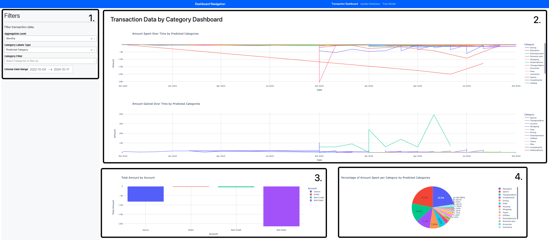
Starting off, let’s go over the filters (number 1. in the main image):

The Aggregation Level filter is used for the time trend and it aggregates the transaction amounts into different levels. The levels are monthly, weekly, daily, or yearly. The Category Labels Type is to either see the categorical spending based on the model’s predctions (Predicted Category) or based on my own personal categorization (True Category). As a note, if I did not label a transaction, it will not show up on the dashboard until I label the data. This is much easier to do for Predicted Category as we will get to when we move onto the update_database_page. Next, we move onto the Category Filter this will allow me to choose certain categories to see further data more in depth. By default, I see all the categories. Finally, the Choose Date Range filter will allow me to modify the max and min time period to view the data. By default, it chooses the max and min dates in the database and the filter will not allow the user to look at data beyond that range.

Moving on to the main content of the page. We first begin with the time trends (labelled as 2. on the main picture), this plot has two different time trends, where the transaction amounts are aggregated based on the Aggregation Level filter. The top time trend is the amount I spend in a given month while the bottom time trend is the amount I gained in a given time period. Next, labelled as 3. in the main picture, I wanted to visualize the total amount per source. As a result, the bar plot is the sum of all transactions for each institution (BoA, AmEx, and Venmo). There are four categories, because I have both a checking account and a credit account with Bank of America. Finally, the last plot (labelled as 4.), is a simple pie chart to show how much I spent on each category within the given time period.

Store Data and Predict Categories

Moving onto the Update Database page, this page can be viewed in four distinct sections viewed in the picture below (I have blacked out some of the data on the DataTable for privacy purposes on my transaction information):

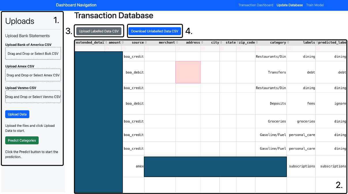
Starting out with the first section, the sidebar is the main location to upload any new data or modify any of the rows of the data. The user will upload .csv files for each of the different banks by either dragging and dropping the file into the respective institution that is labelled or the user can click on the institution to select from their files. Once the data is selected and ready to be stored in the database, the user can then press “Upload Data” which will then either replace any already existing transactions or add new rows, based on the primary key transaction_id. Once the data is uploaded, the user can then click the Predict Categories button to load the saved ensemble model and predict any unlabelled categories. By viewing the DataTable in number 2. of the image above, there are two final columns labels and predicted_labels. The predicted_labels are the categories determined by my custom model while the labels is manually labelled by myself.

Moving onto the DataTable, the table displays all transaction data from the transactions database updates whenever the page refreshes. This will allow you to view whether the new data was successfully updated and predicted. Another useful feature with the DataTable is the ability to multi sort the columns by clicking the column names to which the user wants to sort by. Underneath the sort buttons/column names, there is also a filter option where the user can query transactions based on words that they type into there.

Finally, sections 3. and 4. is to update the labels column of the data. Now, you only need to do this if you are looking to retrain your model or want updated accuracy numbers. The Download Unlabelled Data CSV button (labelled as number 4.) will download any rows where the labels column is null into a .csv file. The user will then label the data by typing which transaction goes into which category. Once completed, the user will then press the Upload Labelled Data CSV and select the labelled transaction data. This will then update the database based on the transaction_id, which the user can review after they refresh the page.

Train Model

Once all the data is now labelled and uploaded, I will want to occasionally train my model and update it based on the results of the new training. This leads us to the Train Model page of the app, where we can review the metrics of the model and choose to train a new model or not.

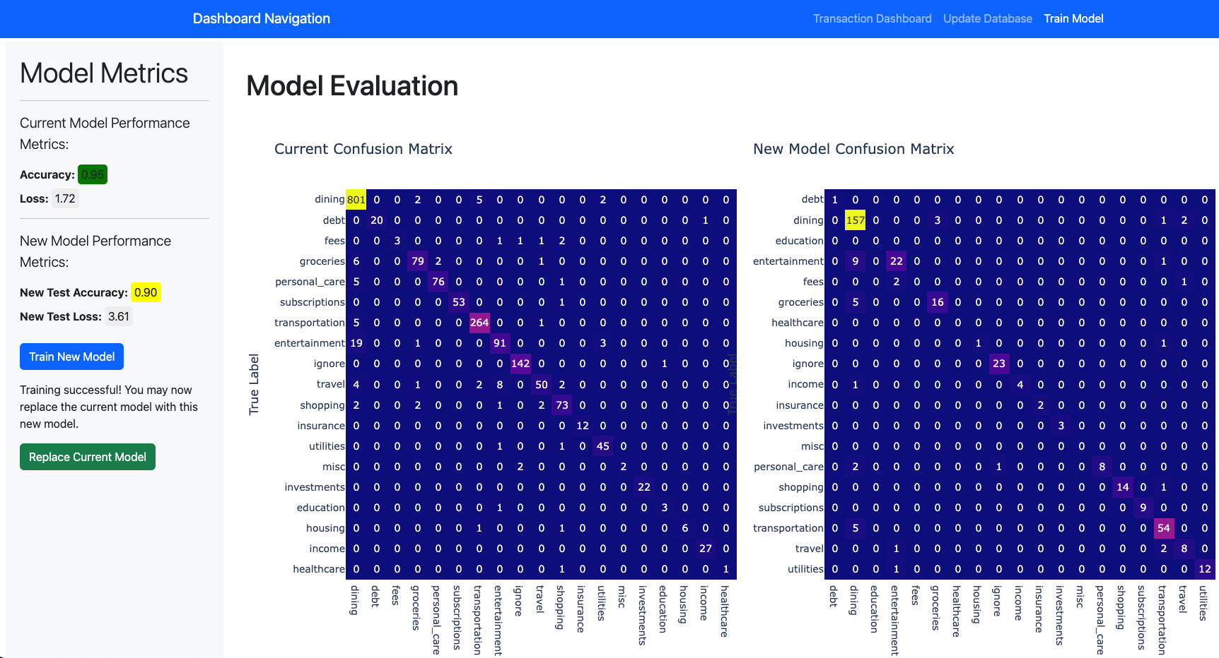
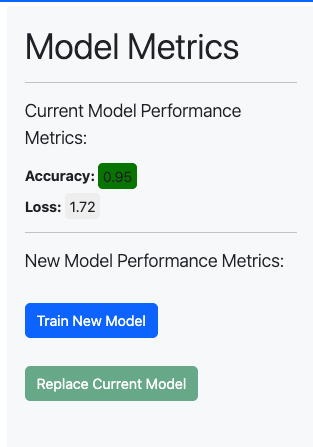
The sidebar now shows the Current Model Performance in terms of the total accuracy and loss. The user can thus press the Train New Model button which will go about the process of training a model. Once the model is trained, a new confusion matrix, test accuracy, and test loss will be displayed as seen in the picture above. Also, when the new model is trained a message will appear and the Replace Current Model button will be enabled (you can see how the button is disabled prior to training in the picture below). The user can then select that button to save the new model in a \current_model directory, thus replacing it. If the user does not want to replace the model, they simply need to refresh or exit the page.

As stated previously, the main content of the page will show a confusion matrix of the current and new models in order to calculate precision and recall. If the user scrolls down further, there will also be a bar plot that shows the distribution of the true categories vs predicted categories for the current and new models. This will show how close the distributions actually are.

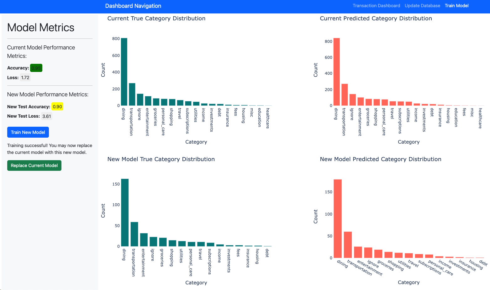
Just as a note, the new model that I trained has a low accuracy and a higher loss because I only trained for 5 epochs for my neural network to speed up training for visualization purposes. I have since updated that back to 1000 epochs with an early_stopping callback.

Conclusion

There is still much more I need to develop with this app. Some further steps I need are as follows:

• Need more metrics for the current and new models for better understanding of the performance.
• Create a loading screen for the train model button in order for the user to know the progress (training the model takes several minutes)
• Determine if there are comparable performance embeddings that take less compute (currently DistilBert still takes around 2 minutes to embed the text data)
• Collect more data and update the database/models
• Make the app nicer and potentially review if this should be hosted somewhere online as opposed to on my local computer

Overall, this was a very fun and useful project to me that showed me a small version of the end to end process for creating a machine learning classification model. I hope to apply this in other applications and increase the complexity of my current one over time!