Sustainable Food Delivery Service

Throughout the course of my Fundamentals of Data Engineering class, we have been developing creating a delivery service for our hypothetical company called AGM (Acme Gourmet Meals). Prior to starting this project, we created PostgreSQL relational tables that stored customer data and stores data. For this final project, we were to create a NoSQL Neo4j database for an open-ended project with any of the data from the relational tables.

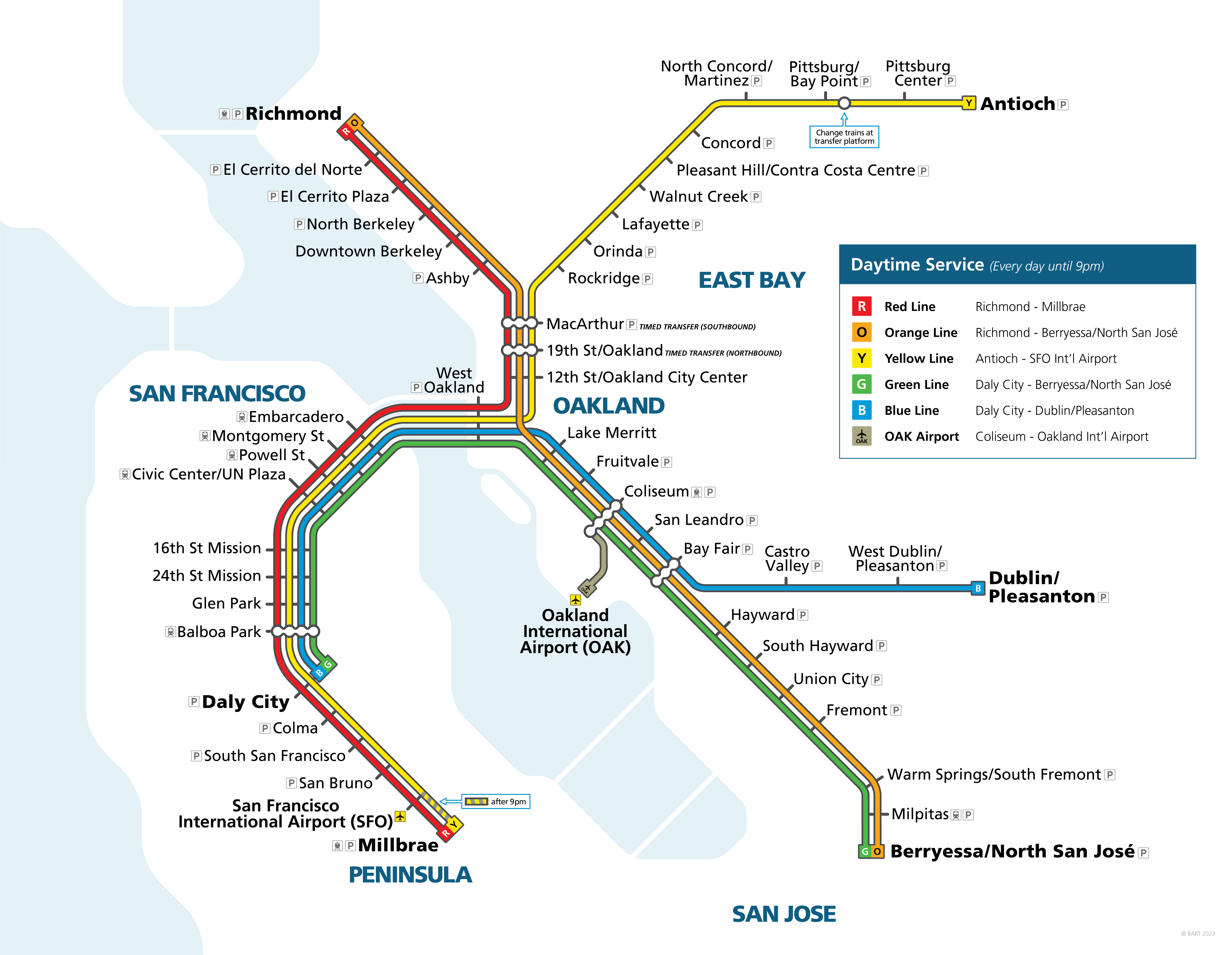
For my project, I used Neo4j to build a graph database to begin the development of a delivery service in the Bay Area. The graph database would consist of customer nodes, store nodes, and station nodes, where the station nodes were representative of the different stations for BART. To add extra challenge to this project, I decided to create a delivery survice that was eco-friendly and so all transportation services would either be through BART or by e-bike to go from a store to a customer.

Below is the high level layout of our graph database, where store_id, store [lat,long], customer_id, and customer [lat,long] were given through relational databases, where [lat,long] is the latitude and longitude coordinates. The station nodes were compiled into a csv and stored in a relational database. Each station was comprised of several nodes, representing the different colored lines on BART. They stations were related by transfer and commute times, where the tranfer time is the average time to transfer from one line to another at the same station, and commute time is the average time to go from one station to the next station.

The two main pieces of information that we did not have were the time to e-bike from one node to another and also the customer [lat,long] coordinates. The customer [lat,long] coordinates were based off a random coordinate within a geodesic box, using the geographiclib.geodesic library, shown in the code below:

def my_calculate_box(point, miles):
    "Given a point and miles, calculate the box in form left, right, top, bottom"
    
    geod = Geodesic.WGS84

    kilometers = miles * 1.60934
    meters = kilometers * 1000

    g = geod.Direct(point[0], point[1], 270, meters)
    left = (g['lat2'], g['lon2'])

    g = geod.Direct(point[0], point[1], 90, meters)
    right = (g['lat2'], g['lon2'])

    g = geod.Direct(point[0], point[1], 0, meters)
    top = (g['lat2'], g['lon2'])

    g = geod.Direct(point[0], point[1], 180, meters)
    bottom = (g['lat2'], g['lon2'])
    
    return(left, right, top, bottom)

# Find a geographic box for each customer based on the zip code that they live in.
# zip_center_point is the [lat,long] of the central point in the zip code
# zip_box_miles is length of the zip code in miles, based on the area of the zip code
# multiply by np.sqrt(2)/2 to get half diagonal of the square to create the box
customers_df['customer_box'] = customers_df.apply(lambda row: my_calculate_box(row['zip_center_point']
                                                                            ,row['zip_box_miles']*np.sqrt(2)*0.5),axis=1)

# create a random latitude and longitude for each customer based on the box created
customers_df['lat_long'] = customers_df.apply(lambda row: (random.uniform(row['customer_box'][3][0]
                                                                            ,row['customer_box'][2][0])
                                                                ,random.uniform(row['customer_box'][0][1]
                                                                            ,row['customer_box'][1][1]))
                                                    ,axis = 1) 

The e-bike times were created with the Google Maps Directions API using the [lat,long] coordinates of all the nodes. Then we applied this to all the customers and stores to connect them to Bart Stations and to one another. Google Maps Directions gave us the durations between two nodes via biking; however, since we were using e-bikes, we applied a coorection factor of 1.5, assuming that e-bikes were 50% faster than normal bikes. This assumption is reasonable since e-bikes can have maximum speeds of up to 28 mph, which is double the speed of a normal bike. The code for the functions and application are shown below:

def google_api_bike_travel_time(api_key, origin, destination):
    """Use Google Maps API for a given key to get the biking travel time between the origin [lat,long]
    and the destination [lat,long]. Divides  that travel time by the e_bike_factor, correcting for the speed
    of an e-bike over normal biking."""
    base_url = "https://maps.googleapis.com/maps/api/directions/json?"
    params = {
        'origin': f"{origin[0]},{origin[1]}",  # Latitude, Longitude
        'destination': f"{destination[0]},{destination[1]}",  # Latitude, Longitude
        'mode': 'bicycling',
        'key': api_key
    }
    
    response = requests.get(base_url, params=params)
    directions = response.json()
    
    # assume e-bikes are 50% faster than normal bikes
    e_bike_factor = 1.5
    
    if directions['status'] == 'OK':
        route = directions['routes'][0]
        leg = route['legs'][0]
        duration = leg['duration']['value'] 
        return duration / e_bike_factor
    else:
        return "Invalid Location"


def find_biking_time(thing,store_or_bart="bart",manual=0):
    """Used to find conduct the API call to find the biking times between a thing and either to the bart or to
    the store. Only used for the .apply() function on a pandas dataframe."""
    if store_or_bart == "bart":
        origin = thing['lat_long']
        destination = thing['nearest_bart_lat_long']
    elif store_or_bart == "store":
        origin = thing['lat_long']
        destination = thing['nearest_store_lat_long']
    return google_api_bike_travel_time(my_api_key,origin,destination)

customers_df['nearest_store_bike_time_seconds'] = customers_df.apply(lambda row: find_biking_time(row,"store"),axis=1)
stores_df['nearest_bart_bike_time_seconds'] = stores_df.apply(lambda row: find_biking_time(row,"bart"),axis=1)

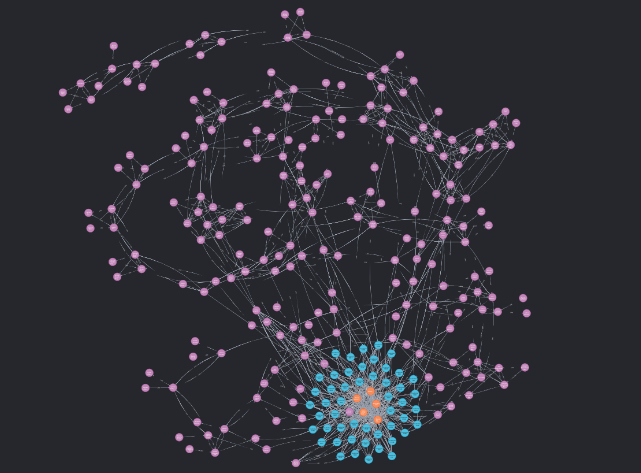
With the relationships between all stores, customers and nodes added, we then connected stored each of the nodes and related each of the nodes by the corresponding travel times between nodes. The final graph database can be seen in the below figure:

Although there are 5 store nodes in the graph, we originally started with one store node that was nearest to the Ashby BART station. We analyzed this graph with Louvain Modularity community detection algorithms and betweenness algorithms to determine which stations were in communities and within each community, which station had the lowest betweenness. To use the graph algorithms in Neo4j, we first create a graph project with the code below:

# drop any existing projects first
query = "CALL gds.graph.drop('ds_graph', false)"
session.run(query)

query = """

CALL gds.graph.project('ds_graph',['Station','Store','Customer'], 'LINK', 
                      {relationshipProperties: 'weight'})
"""

session.run(query)

To find the communities with Louvain Modularity and the betweenness of all nodes, we used the gds.louvain.stream function on our 'ds_graph' project. We then collected the data into DataFrames using the my_neo4j_run_query_pandas() function:

def my_neo4j_run_query_pandas(query, **kwargs):
    "run a query and return the results in a pandas dataframe"
    
    result = session.run(query, **kwargs)
    
    df = pd.DataFrame([r.values() for r in result], columns=result.keys())
    
    return df

query = """

CALL gds.louvain.stream('ds_graph', {includeIntermediateCommunities: true})
YIELD nodeId, communityId, intermediateCommunityIds
RETURN gds.util.asNode(nodeId).name AS name, communityId as community, intermediateCommunityIds as intermediate_community
ORDER BY community, name ASC

"""

station_modularity = my_neo4j_run_query_pandas(query)

query = """

CALL gds.betweenness.stream('ds_graph', {relationshipWeightProperty: 'weight'})
YIELD nodeId, score
RETURN gds.util.asNode(nodeId).name AS name, score as betweenness
ORDER BY betweenness DESC

"""

betweenness_df = my_neo4j_run_query_pandas(query)

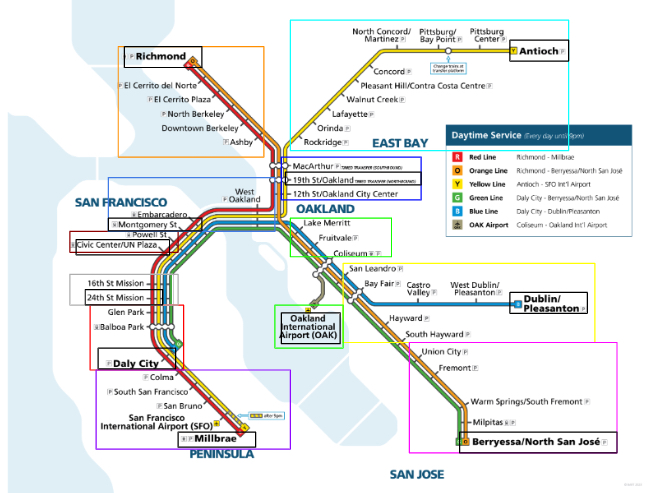
The results of our project is shown below, where each different colored box is a different community calculated by the Louvain Modularity algorithm. We wanted to find potential new store nodes that we could add. As a result, we utilized the betweenness algorithm to find the nodes within each community with the lowest betweenness. We chose the lowest betweenness because these nodes could be interpreted as the stations that took the longest to get to by any other node and so having a store location there could assist the customers located nearest that BART station retrieve their meals faster. The boxes in black represent the station in each community with the lowest betweenness. In total, this resulted in 11 total communities, which would mean adding 10 new stores since we already have a store by the Ashby BART station.

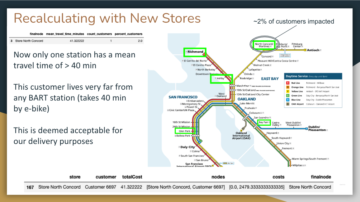
Finally, to go one step further, I asked if it was possible to reduce the number of store locations from 10 new stores down further. In order to do so, I used Dijkstra’s shortest path to find the shortest path from our current store node to all of our customers. What I wanted to determine were which locations took longer than 40 minutes to e-bike or BART to. We chose 40 minutes as that is typically the amount of time that you would have to wait for any normal delivery service. This resulted in 11 different stations; however, by reviewing where these stations were, we could group them into four distinct clusters that we should be able to cater to if we put a store in any of those clusters. As a result we were able to choose one node from each of these four clusters to add a store and recalculate. After recalculating the shortest path from each store to all customers, we saw that we were now able to reach our whole customer base within 40 minutes, except for one individual, who lived exceptionally far from any BART station, even by e-bike. However, because this customer was only 41 minutes away from our new store by e-bike, we deemed this as acceptible as it is not egregiously over the threshold.

In conclusion, we recommended there to be four new stores at North Concord, Richmond, Glen Park, and Bay Fair in order to reach our customers quickly and in an environmentally friendly manner. Overall, this project showed me the significance of NoSQL graph databases compared to traditional relational databases. Without complex joins, we could perform complex algorithms nearly instantaneously which would not be possible in a traditional SQL. Further improvements can be made with this graph such as having a function that can constantly call the google API to update travel times. Also adding nodes with biking paths can make a more granular app that can be seen as a traditional maps app.